
How Nearby Construction Affects Your Property Value
We matched 415 suburb pairs and proved it: a wave of apartment construction caused 4.3% less growth over three years. Not all supply is equal. Apartments drag prices. New houses help neighbours.
 Luke Metcalfe · Microburbs Research · March 2026
The Bottom Line
415 matched suburb pairs. The ones hit by apartment construction grew 4.3% less than their twins.
We matched suburbs that received a sudden wave of 200+ new apartments against similar suburbs that avoided one. Same city. Similar prices. Similar transport access. Three years later, the apartment-hit suburbs had grown 4.3% less. In Sydney, the gap was 7.1%. In Melbourne, 5.8%.
Cross-sectional data supports this. Suburbs surrounded by less construction grew 1.9% faster per year. On a $1M property over 10 years, that raw gap compounds to $309,000. However, part of that gap reflects location quality. Low-supply suburbs tend to be established, well-connected areas. After adjusting for CBD distance, income, and infrastructure, the effect shrinks by about 40% but remains meaningful.
We counted every new home built in Australia since 2016. Houses, apartments, townhouses. 4.48 million in total. For each area, we checked how much construction happened within 7 km. Then we compared price growth.
Why 7 km? When buyers compare suburbs, they look at places within about a 10-minute drive. That is roughly 7 km. Close enough that new apartments in the next suburb compete for the same pool of buyers.
The Results, City by City
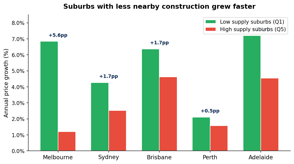
The pattern shows up in every major capital. Melbourne has the strongest raw gap. Adelaide has the weakest. Note: these are raw quintile gaps. Part of the difference reflects location quality rather than supply alone. After adjusting for CBD distance, income, and infrastructure, the gaps narrow by roughly 40%.
| City | Low Supply Growth (per year) | High Supply Growth (per year) | Gap |
|---|---|---|---|
| Melbourne | 6.86% | 3.58% | +3.28% |
| Perth | 3.59% | 1.55% | +2.04% |
| Sydney | 7.32% | 5.43% | +1.89% |
| Brisbane | 4.93% | 3.30% | +1.64% |
| Adelaide | 5.63% | 4.79% | +0.84% |
Low supply = bottom 20% of suburbs by nearby construction within 7 km. High supply = top 20%.
In Melbourne, the gap is 3.28%. A $900,000 house in a low-supply suburb like Eltham would grow $29,500 more per year than the same house in a high-supply suburb. Over a decade that compounds to roughly $400,000.
Distance Matters
How far away does construction need to be before it stops affecting your suburb? We tested five different radiuses across all capital cities.
| Radius | Low Supply Growth | High Supply Growth | Gap |
|---|---|---|---|
| 3 km | 5.68% | 5.10% | +0.58% |
| 5 km | 5.82% | 5.04% | +0.78% |
| 7 km | 5.91% | 5.04% | +0.87% |
| 10 km | 5.95% | 5.07% | +0.88% |
| 15 km | 5.87% | 5.07% | +0.80% |
The effect peaks around 7 to 10 km. Construction more than 15 km away has less impact. But even buildings 3 km away create a measurable drag on growth.
What Type of Construction Hurts Most?
Not all construction affects your suburb the same way. Apartment towers and house-to-unit conversions drag on nearby prices. But new houses in surrounding areas are actually linked to higher growth for neighbours.
| Type of Construction | Low Supply Growth | High Supply Growth | Gap |
|---|---|---|---|
| New houses nearby | 4.73% | 6.49% | -1.76% |
| Apartment towers nearby | 5.88% | 4.63% | +1.25% |
| House-to-unit conversions | 6.14% | 4.63% | +1.51% |
When both unit supply and house supply appear in the same regression model, they carry opposite signs in four of five capitals. This is a key finding. Apartment construction within 7 km is associated with 1 to 3 percentage points lower annual growth. House construction signals growing demand, infrastructure investment, and expanding amenity. Unit-dominated suburbs grew just 4.63% per year on average. House-dominated suburbs grew 6.49%.
The worst combination: suburbs near both apartment towers and house-to-unit conversions. These areas face a double supply hit. Think inner-ring Melbourne suburbs like Burnley and Travancore, surrounded by towers in every direction.
Cause and Effect: The Strongest Evidence
The city-by-city patterns above are suggestive, but they could partly reflect location quality. Low-supply suburbs tend to be established, desirable areas. So we ran a tougher test.
We matched 415 suburbs that received a sudden wave of 200 or more new apartments against similar suburbs that avoided the construction. Same city. Similar prior prices and growth trends. Similar transport access. The only difference was the building wave.
Three years later, the suburbs with new apartment towers had grown 4.3% less than their matched controls.
| City | Matched Pairs | Impact on Growth (3 years after construction) |
|---|---|---|
| Sydney | 165 | -7.1% |
| Melbourne | 60 | -5.8% |
| Brisbane | 46 | -4.0% |
| All capitals | 415 | -4.3% |
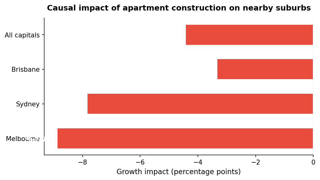
Larger shocks produced larger effects. Suburbs receiving 300+ new units saw a steeper penalty than those receiving 200 to 299. This dose-response gradient is consistent with a causal mechanism.
Here are two real examples from those 415 matched pairs.
Abbotsford (Vic) vs Canterbury (Vic)
Abbotsford received 463 new units. Prices fell 3%. Canterbury, a comparable suburb without the construction wave, grew 16.6%. That is a gap of 19.6%.
Annandale (NSW) vs Haberfield (NSW)
Annandale received 658 new units. Prices fell 8.4%. Haberfield, a nearby suburb that avoided the building wave, grew 11.7%. That is a gap of 20.1%.
This is not just a pattern. The before-and-after study across 415 matched suburb pairs confirms that apartment construction causes slower growth. This is the strongest evidence in the study.
Two Sydney Suburbs, Two Very Different Outcomes
Both are unit markets in Sydney. But Dee Why had low nearby construction. Zetland had 185,000 new properties built within 7 km. Dee Why units grew roughly 20%. Zetland went sideways for seven years.
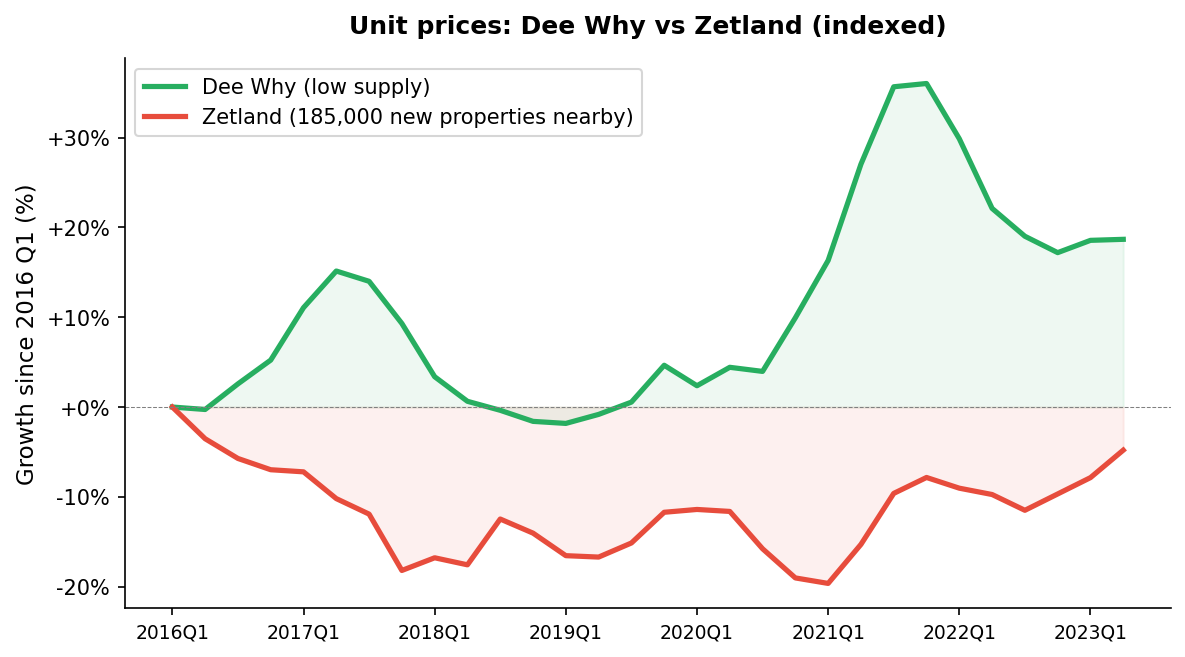
Dee Why sits on the Northern Beaches, surrounded by national park and low-density suburbs. Very little new construction within 7 km. Unit prices rose from $715,000 to $880,000.
Zetland sits in the middle of Sydney's biggest apartment construction zone. Green Square, Mascot, Waterloo, and Alexandria added tens of thousands of new units nearby. Prices flatlined at around $950,000 for seven years.
Where Is the Construction? A Castlecrag Case Study
On Sydney's Lower North Shore, 95% of new construction is apartments. Here is what went up within 7 km of Castlecrag since 2016. Each tower adds competing stock that buyers can choose instead of an established home nearby.
| Locality | Units | Houses | Total |
|---|---|---|---|
| North Sydney | 5,574 | 275 | 5,849 |
| Chatswood | 4,402 | 238 | 4,640 |
| St Leonards | 3,758 | 108 | 3,866 |
| Mosman | 2,709 | 336 | 3,045 |
| Cremorne | 2,813 | 185 | 2,998 |
| Neutral Bay | 2,364 | 133 | 2,497 |
| Wollstonecraft | 2,362 | 96 | 2,458 |
| Lane Cove | 2,180 | 142 | 2,322 |
| Artarmon | 1,956 | 87 | 2,043 |
| Crows Nest | 1,842 | 64 | 1,906 |
Real Suburb Examples
Eltham, Vic
$785K to $1.015M in 7 years (3.7% per year)
Low nearby supply. Established suburb near a train station. Surrounded by green wedge land where construction is restricted. Few new properties within 7 km means less competition from new stock.
Epping, Vic
$412K to $635K in 7 years (6.4% per year)
Outer northern suburb with surprisingly low surrounding supply. Despite being on the urban fringe, the nearby areas had modest construction compared to western Melbourne. Strong growth followed.
Burnley, Vic
$530K dropped to $525K
Surrounded by unit towers along the Yarra. Thousands of new apartments in neighbouring Richmond, Cremorne, and South Yarra created heavy competition for buyers.
What About Regional Areas?
In small regional towns, there is no supply drag at all. The pattern actually flips. High-supply regional suburbs grew 9.1% per year compared to 7.4% for low-supply areas. New construction in a small town signals jobs arriving and a community on the rise.
But larger regional centres tell a different story. Once a town is big enough to have competing areas, the capital city pattern starts to appear.
Larger centres with a supply drag
Townsville shows the strongest regional effect. Suburbs there with the most nearby construction grew just 1.1% per year compared to 3.5% for low-supply areas. Geelong and Toowoomba follow the same pattern as capital cities: more nearby building, slower price growth.
Coastal corridors flip positive
The Gold Coast, Sunshine Coast, and Cairns are the opposite. In these coastal corridors, construction follows demand. New homes going up is a sign the area is booming, not that it is oversupplied.
Results by Region
Every region in Australia behaves differently. We grouped them into five types.
Capital Cities
More construction nearby generally means slower growth. Strongest in Melbourne and Perth.
| Region | Suburbs | Effect | Low Supply | High Supply | Impact |
|---|---|---|---|---|---|
| Sydney | 511 | Supply drags | 7.3% | 5.4% | -1.9% |
| Melbourne | 359 | Supply drags | 6.9% | 3.6% | -3.3% |
| Adelaide | 297 | Mixed | 5.6% | 4.8% | -0.8% |
| Perth | 277 | Supply drags | 3.6% | 1.6% | -2.0% |
| Brisbane | 169 | Supply drags | 4.9% | 3.3% | -1.6% |
| Canberra | 90 | Supply drags | 5.3% | 3.3% | -2.0% |
| Darwin | 28 | Mixed | 0.7% | 0.7% | -0.1% |
| Hobart | 24 | Supply drags | 10.5% | 9.1% | -1.3% |
Large Regional Centres
Cities big enough to have competing areas. The supply drag appears here too, but weaker than capitals.
| Region | Suburbs | Effect | Low Supply | High Supply | Impact |
|---|---|---|---|---|---|
| Newcastle | 98 | Supply drags | 7.7% | 6.0% | -1.8% |
| Ipswich | 77 | Supply drags | 8.8% | 5.8% | -3.1% |
| Gippsland | 72 | Supply helps | 7.8% | 8.9% | +1.1% |
| Hunter Valley | 62 | Supply helps | 7.7% | 8.8% | +1.1% |
| Wollongong | 52 | Mixed | 6.5% | 6.1% | -0.4% |
| Logan | 52 | Supply helps | 6.7% | 9.7% | +3.0% |
| Townsville | 52 | Supply drags | 3.5% | 1.1% | -2.3% |
| Geelong | 50 | Supply drags | 11.5% | 8.3% | -3.1% |
| Toowoomba | 35 | Supply drags | 10.0% | 7.8% | -2.2% |
| Central Coast | 78 | Mixed | 6.5% | 7.3% | +0.8% |
| Mackay | 39 | Mixed | 4.7% | 5.4% | +0.7% |
| Ballarat | 41 | Mixed | 9.2% | 8.2% | -1.0% |
| Bendigo | 33 | Mixed | 9.4% | 8.9% | -0.4% |
| Albury / Wodonga | 34 | Supply drags | 10.0% | 7.5% | -2.4% |
Coastal and Lifestyle Corridors
Construction here follows demand. New building is a sign the area is booming, not oversupplied.
| Region | Suburbs | Effect | Low Supply | High Supply | Impact |
|---|---|---|---|---|---|
| Sunshine Coast | 94 | Mixed | 11.3% | 10.3% | -1.0% |
| Hervey Bay / Bundaberg | 95 | Supply helps | 6.5% | 8.0% | +1.5% |
| Cairns | 74 | Supply helps | 3.4% | 4.8% | +1.4% |
| Gold Coast | 68 | Mixed | 9.0% | 8.5% | -0.5% |
| Southern Highlands | 44 | Supply helps | 7.7% | 11.4% | +3.7% |
| Port Macquarie | 45 | Supply drags | 10.0% | 8.7% | -1.3% |
| Byron / Tweed | 40 | Supply drags | 10.0% | 7.1% | -2.9% |
| Mornington Peninsula | 34 | Supply helps | 9.1% | 10.3% | +1.2% |
| Bunbury | 43 | Mixed | 4.3% | 4.4% | +0.1% |
| Warrnambool | 20 | Supply helps | 7.5% | 12.8% | +5.3% |
| Coffs Harbour | 25 | Supply helps | 7.9% | 9.1% | +1.2% |
| Mandurah | 20 | Supply helps | -0.3% | 5.5% | +5.9% |
Growth Frontiers
New towns and expanding regions. Supply and growth go hand in hand here.
| Region | Suburbs | Effect | Low Supply | High Supply | Impact |
|---|---|---|---|---|---|
| WA Wheat Belt | 47 | Supply helps | -2.0% | 5.5% | +7.5% |
| Rockhampton / Gladstone | 54 | Supply helps | 1.4% | 5.3% | +3.9% |
| Darling Downs | 26 | Supply helps | 1.6% | 6.4% | +4.7% |
| Redcliffe / North Lakes | 25 | Supply helps | 7.8% | 10.0% | +2.2% |
| Tamworth / Armidale | 25 | Supply helps | 2.9% | 5.6% | +2.7% |
| Griffith / Leeton | 25 | Supply helps | 7.7% | 10.6% | +3.0% |
| NW Tasmania | 25 | Supply helps | 5.3% | 6.5% | +1.2% |
| Shepparton | 14 | Supply helps | 6.5% | 11.5% | +5.0% |
| Dubbo / Broken Hill | 10 | Supply helps | 2.8% | 8.9% | +6.1% |
| Outback Queensland | 20 | Supply helps | -4.5% | 1.2% | +5.6% |
| NT Outback | 10 | Supply drags | 1.3% | 0.1% | -1.2% |
Other Regions
Smaller markets with limited data. Not enough suburbs for a clear pattern in most.
| Region | Suburbs | Effect | Low Supply | High Supply | Impact |
|---|---|---|---|---|---|
| Southern NSW | 48 | Mixed | 10.3% | 10.1% | -0.2% |
| WA South | 46 | Supply drags | 1.6% | -0.3% | -1.9% |
| Mount Gambier | 42 | Supply helps | 6.0% | 7.6% | +1.6% |
| Caboolture / Bribie | 33 | Supply drags | 8.5% | 7.5% | -1.1% |
| Orange / Bathurst | 29 | Supply drags | 8.2% | 7.2% | -1.1% |
| Barossa Valley | 29 | Mixed | 3.4% | 3.7% | +0.3% |
| Albury / Wagga | 28 | Supply drags | 8.7% | 6.7% | -2.0% |
| Launceston | 21 | Mixed | 9.6% | 9.5% | -0.1% |
Microburb Maps
These interactive maps show exactly where supply is concentrating. Each one focuses on a different area. The colour shading shows how much new construction happened in each Microburb.
Supply vs Growth: The Full Picture
Every dot is an area. The horizontal axis shows new properties within 7 km. The vertical axis shows annual price growth from 2016 to 2025. The downward slope tells the story.
The interactive scatterplot is available in the full whitepaper. Read the whitepaper →
Micropocket Map
This map highlights areas with historically low nearby supply. These "micropockets" are places where geography, zoning, or green wedge boundaries restrict surrounding construction.
The interactive micropocket map is available in the full whitepaper. Read the whitepaper →
What This Means for You
Check what type of construction is within 7 km
Before buying, look at construction activity in surrounding areas. Apartment towers compete for the same pool of buyers. But new houses nearby are a positive signal. Not all supply is equal.
Apartment supply drags growth. House supply helps.
When both appear in the same model, they carry opposite signs in four of five capitals. Apartment construction within 7 km is associated with 1 to 3 percentage points lower annual growth. New house construction lifts neighbour returns by 1.76%.
The causal evidence is strong
415 matched suburb pairs showed a 4.3% growth penalty from apartment construction shocks. In Sydney, the penalty was 7.1%. In Melbourne, 5.8%.
Supply is one factor among many
With all controls, supply explains about 3.7% of suburb growth variation. The raw 1.9% annual quintile gap shrinks by 40% after adjusting for CBD distance, income, and infrastructure. The effect is real but modest.
Look for natural supply barriers
Green wedge zones, national parks, waterfront, and heritage overlays all restrict future construction. Suburbs surrounded by these barriers, like Eltham and Dee Why, have historically outperformed.
Regional towns are different
In smaller centres, new construction is a growth signal, not a drag. The supply effect only appears once a town is large enough to have competing areas within a few kilometres.
Read the Research
The full whitepaper covers methodology, infrastructure controls, and detailed city-by-city breakdowns.
Read the ResearchRead the Research