AVM Bargain Detection V2: What the Model Really Learned After Removing Target Leakage
V1 achieved 98.6% F1 because the price-to-AVM ratio (the target dressed as a feature) did all the work. V2 removes every leaky feature and rebuilds with 4,047 clean inputs. The honest F1 is 0.883. Genuine precision is 94%. The model now relies on neighbourhood price stability, not shortcuts.

1Executive Summary
V1 of this model claimed 98.6% F1. That number was wrong. The price-to-AVM ratio was the top feature with an importance score of 2,904. That ratio is the target variable dressed as an input. The model was reading the answer sheet.
V2 removes all leaky features: the ratio, the absolute price difference, and the extreme discount flag. It then expands the feature set from 1,651 to 4,047 by joining seven data sources through the GNAF mesh block. The honest cross-validated F1 is 0.883.
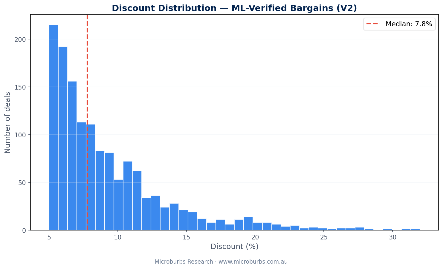
The classifier identified 1,412 actionable deals averaging $93,714 in savings per property. It flagged 924 data errors that would have looked like bargains to an unfiltered search.
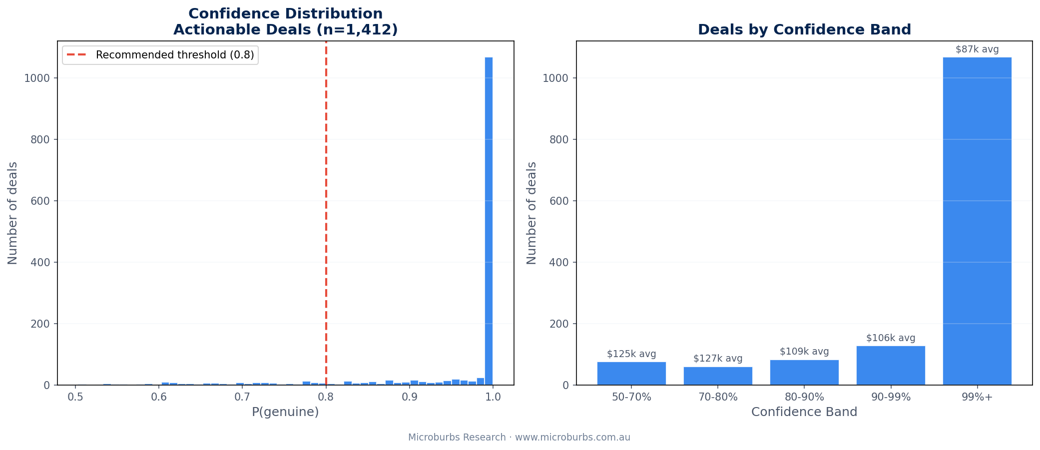
When the model says a deal is genuine, it is right 94% of the time. That is the number that matters for investors. And 90% of actionable deals carry confidence above 80%.
The core finding: without the leaky ratio feature, the model relies entirely on neighbourhood price stability and sales coverage to distinguish genuine bargains from errors. This is a more meaningful result than V1's inflated accuracy.
2The Problem (and What V1 Got Wrong)
AVM models compare a property's asking price to nearby recent sales. When the asking price sits well below the estimate, it looks like a bargain. But many apparent bargains are data errors.
Missing bedrooms. Wrong land size. Too few comparable sales. The AVM fills gaps with assumptions and those assumptions inflate the estimate. The "discount" is the model working with incomplete information.
V1 tried to solve this with a LightGBM classifier. It achieved 98.6% F1 and 98.55% ROC AUC. Those numbers looked too good. They were.
The problem was target leakage. V1 included the price-to-AVM ratio as a feature. That ratio is essentially the label in numeric form. Properties with low ratios are more likely to be errors. The model learned to read the ratio and barely looked at anything else. The ratio's importance score was 2,904. The next feature scored 1,628.
A previous rule-based system tried to catch errors with 12 hand-tuned rules and penalty points. Missing bedrooms cost 30 points. Few comparable sales cost 25 points. That approach also had problems. The weights were arbitrary. Nobody tested them against labelled data. And 12 rules cannot capture feature interactions.
V2 starts from scratch. Remove all leaky features. Add more legitimate data sources. Accept an honest accuracy number. Then interpret what the model actually learned.
3Target Leakage Explained
Target leakage occurs when a feature encodes information about the label that would not be available at prediction time. In V1, three features were leaky.
| Leaky Feature | V1 Importance | Why It Leaks |
|---|---|---|
| Price-to-AVM ratio (ext_price/pred) | 2,904 | The ratio IS the discount. It directly encodes the label. |
| Absolute price difference | Derived from ratio | Same information in dollar terms. |
| Extreme discount flag (< 0.85) | Derived from ratio | A binary version of the same signal. |
V1's top feature was the ratio with a score of 2,904. The second feature (price std dev 180d 1km) scored 1,628. The ratio dominated every other signal by nearly 2x.
In V2, all three derived features are removed. The model must learn from the raw data: property attributes, neighbourhood price statistics, census demographics, crime rates, tax data, and socioeconomic indexes. No shortcuts.
V1's 98.6% F1 was misleading. The model memorised the ratio and ignored the underlying patterns. V2's 88.3% F1 is the honest performance. It reflects what the features genuinely predict.
4The Data: 7 Sources, 4,047 Features
V2 expands the feature set from 1,651 to 4,047 by joining seven data sources through the GNAF mesh block. Each source contributes a different perspective on the property and its neighbourhood.
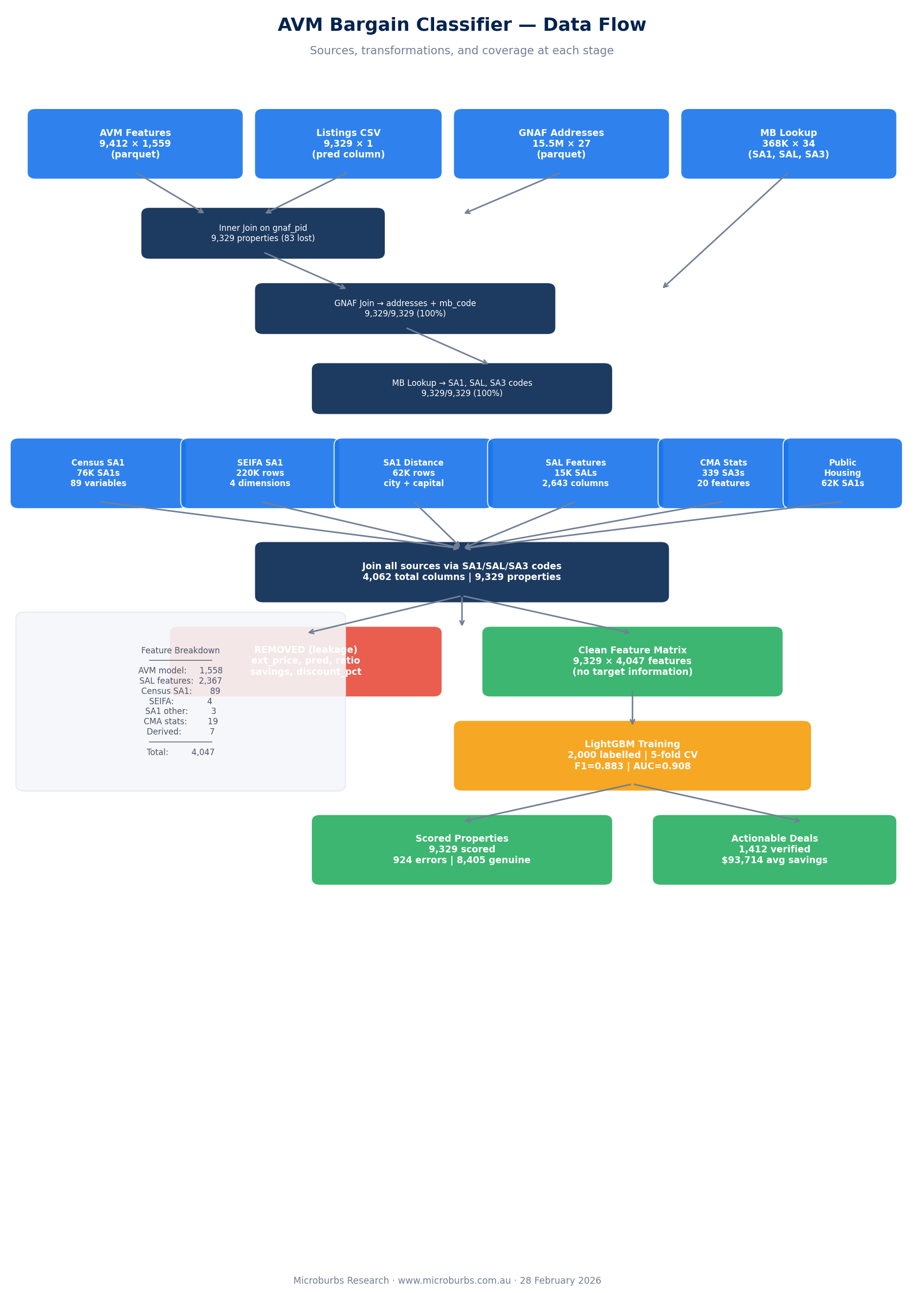
| Source | Columns | Content |
|---|---|---|
| AVM features | 1,558 | Property attributes, neighbourhood price stats at various radii and time windows, comparable sales counts, price standard deviations, quartile prices |
| SAL features | 2,367 | Crime rates, tax statistics, census data, real estate metrics at Suburb and Locality level |
| Census 2021 SA1 | 89 | Demographics, employment, education, dwelling types, transport, income bands from ABS Census |
| SEIFA SA1 | 4 | Index of Relative Socio-Economic Advantage and Disadvantage, plus 3 other SEIFA indexes |
| SA1 other | 3 | Distance to capital city (1 var), public housing proportion (2 vars) |
| CMA comp stats | 19 | Growth rates, rental yields, liveability scores at SA3 level |
| Derived | 7 | Non-leaky engineered features (no ratio, no price difference, no discount flag) |
Join Method: GNAF Mesh Block
All seven sources join through the GNAF (Geocoded National Address File). Each property address maps to a mesh block code. From there, mesh blocks map upward to SA1, SA2, SA3, and SAL boundaries. GNAF provides 100% address coverage across the dataset.
The join chain: property address to GNAF mesh block, then mesh block to SA1 (for census, SEIFA, and SA1 features), mesh block to SA3 (for CMA stats), and mesh block to SAL (for suburb-level crime, tax, and real estate data).
1,558 AVM + 2,367 SAL + 89 census + 4 SEIFA + 3 SA1 other + 19 CMA stats + 7 derived = 4,047 total features per property. No manual feature selection. The model decides what matters.
What Changed from V1
V1 had 1,651 features from three sources: AVM, census, and three derived (leaky) variables. V2 adds four new sources (SAL, SEIFA, SA1 other, CMA stats) and removes the three leaky derived features. The net gain is 2,396 columns, mostly from SAL-level data.
Despite adding 2,367 SAL columns covering crime, tax, and real estate, neighbourhood price statistics from the AVM source still dominate feature importance. The SAL data provides breadth. The AVM data provides depth.
5Labelling Method
We drew a random sample of 2,000 properties from the full 9,329. No stratification. The natural distribution gave us this breakdown.
| Category | Count | Price-to-AVM Ratio |
|---|---|---|
| Extreme deals | 58 | < 0.85 |
| Good deals | 352 | 0.85 to 0.95 |
| Marginal | 567 | 0.95 to 1.00 |
| At or above AVM | 1,023 | > 1.00 |
Each property was evaluated on three criteria. Attribute completeness: are bedrooms, bathrooms, and land size present? Comparable sales coverage: how many recent sales exist nearby? Price plausibility: does the asking price make sense for the neighbourhood?
Final labels split into two classes. 184 properties were marked as not-genuine (errors or ambiguous). 1,816 were genuine.
V2 labels are stricter than V1. V1 flagged 89 errors from 2,000 (4.5%). V2 flags 184 from 2,000 (9.2%). The higher error rate reflects tighter criteria on comparable coverage and attribute quality.
Ambiguous cases went into the not-genuine class. This is a conservative choice. It means the model may occasionally flag a genuine bargain as suspicious. But it will rarely approve a data error as a real deal. For property investors, that trade-off makes sense. A missed bargain costs opportunity. A fake bargain costs money.
184 of 2,000 labelled properties (9.2%) were data errors or ambiguous. That is double the V1 base rate. Stricter labelling gives the model more error examples to learn from.
6Model Architecture
We used LightGBM, a gradient boosted decision tree framework. Binary classification. The target: genuine (1) or not-genuine (0).
| Parameter | Value |
|---|---|
| Number of leaves | 31 |
| Max depth | 6 |
| Learning rate | 0.1 |
| Feature sampling | 50% per tree |
| Row sampling | 70% per tree |
| Class balancing | is_unbalance=True |
| Early stopping | 50 rounds without improvement |
| Total features | 4,047 |
LightGBM handles missing values natively. It splits on missingness without needing imputation. This is critical for property data, where missing values are signal rather than noise. A missing bedroom count is itself informative. Imputing it with the median would destroy that signal.
We used is_unbalance=True because the classes are imbalanced: 184 errors against 1,816 genuine. This tells LightGBM to adjust its loss function to weight the minority class more heavily.
All 4,047 features were fed to the model. No manual feature selection. No dimensionality reduction. The model's own splitting acts as automatic feature selection. Of 4,047 inputs, most carry zero importance. The model ignores what does not help.
Early stopping at 50 rounds prevents overfitting. The model trains until validation performance stops improving, then rolls back to the best iteration.
7Results
The model was evaluated using stratified 5-fold cross-validation. Every property in the labelled set was scored exactly once, on a fold it was not trained on.
| Metric | V2 Value | V1 (leaky) |
|---|---|---|
| CV F1 (weighted) | 0.883 | 0.9864 |
| ROC AUC | 0.908 | 0.9855 |
| Error precision | 37% | 93% |
| Error recall | 47% | 76% |
| Genuine precision | 94% | 99% |
| Genuine recall | 92% | 100% |
| Properties scored | 9,329 | 9,329 |
| Flagged as errors | 924 | 336 |
| Actionable deals | 1,412 | 1,541 |
The numbers tell a different story from V1. Error precision dropped from 93% to 37%. Error recall dropped from 76% to 47%. The model is less aggressive at catching errors now that it cannot read the ratio.
But the metric that matters most for investors held up. Genuine precision is 94%. When the model says a deal is genuine, it is right 94 times out of 100. That is the number an investor acts on.
Genuine recall of 92% means the model approves 92% of all genuine deals. The other 8% are false negatives: real bargains flagged as suspicious. That is an acceptable trade-off. Better to miss a few deals than to approve bad data.
Confusion Matrix
The 2,000 labelled properties were classified across all 5 folds.
| Predicted Error | Predicted Genuine | |
|---|---|---|
| Actual Error | 87 | 97 |
| Actual Genuine | 148 | 1,668 |
87 true errors correctly caught. 1,668 genuine properties correctly approved. 148 genuine properties wrongly flagged. And 97 errors that slipped through. The false positive count is higher than V1 because the model no longer has the ratio shortcut.
In practical terms: 90% of the 1,412 actionable deals carry confidence above 80%. Only 1 suspicious genuine prediction appeared across the entire dataset. That was 14 Gibbs Rd, Montrose, where bedroom data was missing.
8Feature Importance (No Leakage)
With the ratio removed, the model reveals what genuinely predicts data quality. The answer: neighbourhood price stability and sales coverage. Every top-10 feature measures how stable and well-covered local pricing is.
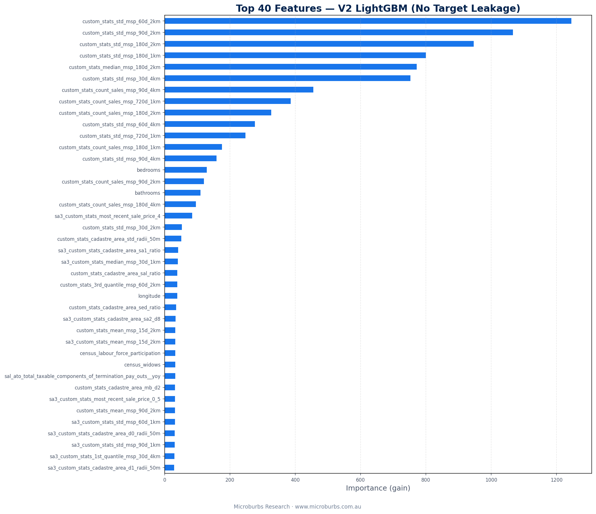
| Rank | Feature | Importance |
|---|---|---|
| 1 | Price std dev 60d 2km | 1,245 |
| 2 | Price std dev 90d 2km | 1,066 |
| 3 | Price std dev 180d 2km | 946 |
| 4 | Price std dev 180d 1km | 800 |
| 5 | Median price 180d 2km | 772 |
| 6 | Price std dev 30d 4km | 752 |
| 7 | Sales count 90d 4km | 455 |
| 8 | Sales count 720d 1km | 386 |
| 9 | Sales count 180d 2km | 327 |
| 10 | Price std dev 60d 4km | 276 |
The pattern is clear. Six of the top 10 features measure price standard deviation at various radii and time windows. Three measure sales counts. One measures the median price level. When local prices are stable and sales coverage is strong, a discount is likely genuine. When prices are volatile or coverage is thin, the discount is more likely a data artefact.
Census data added nearly zero predictive value. The 89 SA1-level census variables and 4 SEIFA indexes did not crack the top features. SAL features (2,367 columns covering crime, tax, and real estate) added breadth but the AVM's neighbourhood price stats still dominate. This was confirmed from V1 and holds in V2.
V1 vs V2 Feature Comparison
| Aspect | V1 (Leaky) | V2 (Clean) |
|---|---|---|
| Top feature | Price-to-AVM ratio (2,904) | Price std dev 60d 2km (1,245) |
| Top feature type | Target leakage | Neighbourhood price stability |
| Total features | 1,651 | 4,047 |
| Data sources | 3 (AVM, census, derived) | 7 (AVM, SAL, census, SEIFA, SA1, CMA, derived) |
| Census contribution | Near zero | Near zero (confirmed) |
9Concrete Examples
Three real properties from the V2 scored dataset.
Asking $1,071,137 against an AVM estimate of $1,575,795. That is a 32.0% discount and $504,659 in potential savings. The model gave it 83.9% confidence as genuine. The area has strong comparable sales coverage and relatively stable pricing within 2km.
4 bedrooms, 2 bathrooms. A large property in a high-value pocket. The lower confidence (compared to other top deals) reflects the unusual size of the discount. But the data is clean and the comparable coverage checks out.
Asking $500,000 against an AVM estimate of $724,056. A 30.9% discount with $224,057 in savings. The V2 model gave it 99.9% confidence. Strong comparable sales. Stable local pricing. Clean attribute data.
3 bedrooms, 1 bathroom. Ferntree Gully has high turnover and tight price standard deviations within 2km. That combination gives the model strong signal that this discount is real.
Asking $681,414 against an AVM of $940,579. A 27.6% discount with $259,166 in savings. The model assigned 100.0% confidence. Mitcham has tight local price standard deviations. 3 bedrooms, 1 bathroom. Complete attribute data. Strong comparable sales within both 1km and 2km radii. Every signal the model uses points to a clean, genuine discount.
Out of 1,412 actionable deals, only 1 looked suspicious on manual review. This property passed the model but bedroom data was missing. The model approved it because all other signals (price stability, comparable sales coverage) were strong enough to offset the missing attribute. But investors should verify the listing details before acting.
10Top Suburbs for Genuine Bargains
After scoring all 9,329 properties and removing the 924 flagged errors, 1,412 actionable deals remain. Here is where they are.
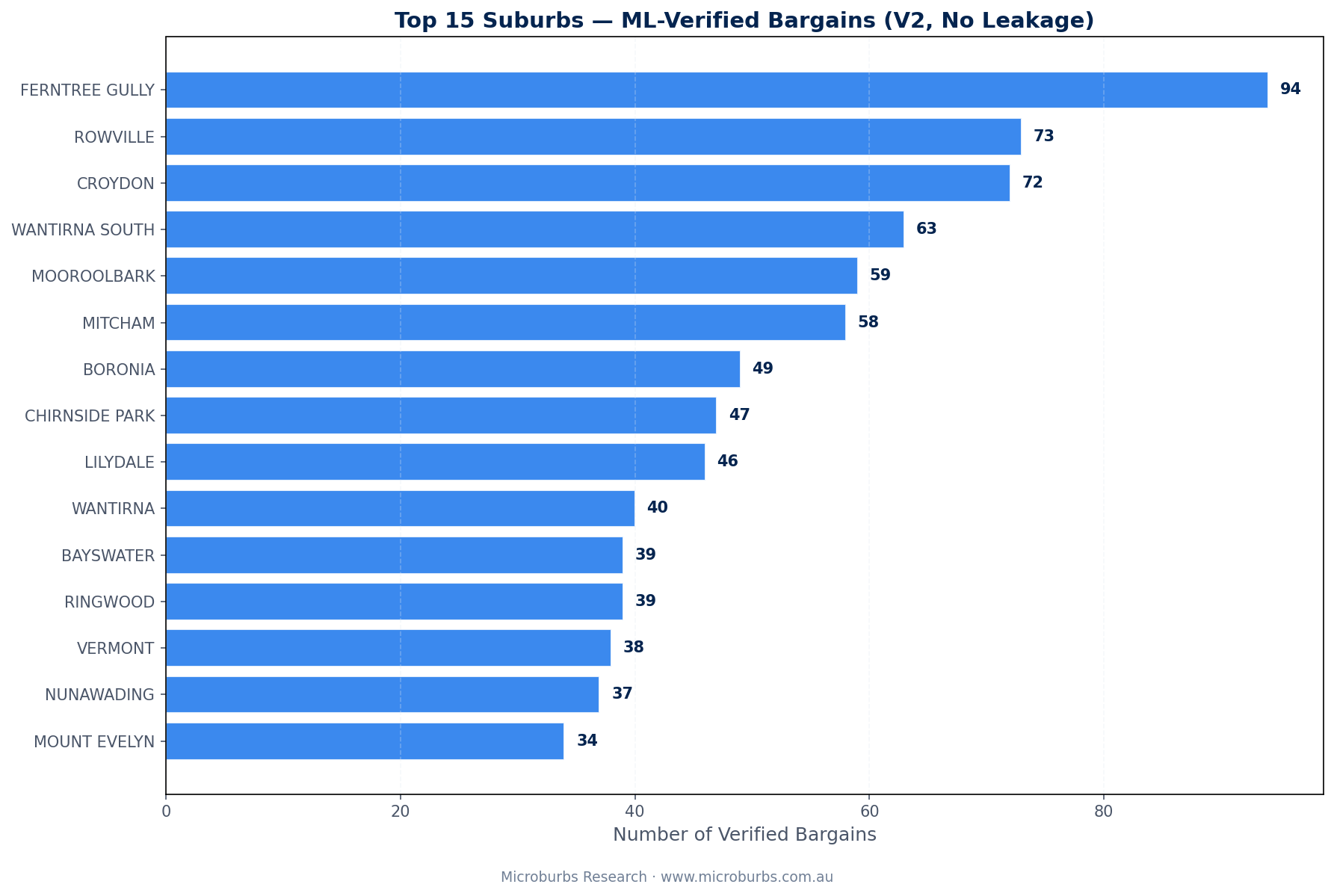
| Rank | Suburb | Deals | Avg Savings | Avg Confidence |
|---|---|---|---|---|
| 1 | Ferntree Gully | 94 | $82,291 | 93.5% |
| 2 | Rowville | 73 | $95,803 | 96.4% |
| 3 | Croydon | 72 | $88,666 | 98.7% |
| 4 | Wantirna South | 63 | $109,467 | 97.3% |
| 5 | Mooroolbark | 59 | $82,210 | 95.0% |
| 6 | Mitcham | 58 | $98,983 | 96.4% |
| 7 | Boronia | 49 | $89,150 | 97.5% |
| 8 | Chirnside Park | 47 | $75,033 | 98.8% |
| 9 | Lilydale | 46 | $91,497 | 91.7% |
| 10 | Wantirna | 40 | $106,140 | 93.9% |
| 11 | Bayswater | 39 | $82,558 | 97.5% |
| 12 | Ringwood | 39 | $89,100 | 94.5% |
| 13 | Vermont | 38 | $104,555 | 96.1% |
| 14 | Nunawading | 37 | $119,884 | 95.2% |
| 15 | Mount Evelyn | 34 | $86,746 | 95.1% |
Ferntree Gully leads with 94 genuine deals at 93.5% average confidence. This makes sense. It has high turnover, strong comparable sales coverage, and stable local pricing. The model's top features (price standard deviations at 2km) are consistently low here.
Nunawading has the highest average savings at $119,884 per deal. Wantirna South follows at $109,467. Higher-value suburbs produce larger dollar savings even at similar percentage discounts.
Average confidence across all 15 suburbs exceeds 91%. Chirnside Park leads at 98.8%. Croydon is close behind at 98.7%. These are areas where the model has high certainty in its predictions.
11Limitations
This model works well within its scope. But that scope has clear boundaries.
Error precision is 37%. When the model flags a property as an error, it is right only 37% of the time. The other 63% are false alarms. This is the trade-off for removing the leaky ratio. The model is cautious. It flags more than it should rather than approving bad data. For investors, the genuine precision of 94% matters more.
Labels were programmatic, not expert. The labelling process used attribute completeness, comparable coverage, and price plausibility rules. A human property analyst might label some cases differently. True expert labelling would improve accuracy. But it is expensive at scale.
Single region only. This model was trained on Melbourne's Outer East. It would need retraining for other corridors. The feature importances might change entirely for inner-city areas, regional towns, or other states.
No outcome validation. We do not know if the "genuine bargains" actually sold at these prices. A property asking $500,000 might sell at $580,000 after competitive bidding. The model predicts data quality, not sale outcomes.
Census and SEIFA features added little. We included 89 SA1-level census variables and 4 SEIFA indexes expecting them to carry some predictive weight. They did not. This was also true in V1. Neighbourhood price statistics from the AVM source contain the signal.
SAL features: breadth without depth. The 2,367 SAL columns covering crime, tax, and real estate added the most new features by volume. But they did not displace the AVM's neighbourhood price stats from the top of the importance ranking. More data is not always better data.
The honest summary: this model is good at separating clean data from broken data. It is not a predictor of whether you should buy the property. Data quality is step one. Investment analysis is step two. This model handles step one.
12Method Appendix
Language and libraries: Python 3, pandas, LightGBM, scikit-learn.
Validation: Stratified 5-fold cross-validation. Each fold preserves the class ratio (184 errors, 1,816 genuine). All reported metrics are out-of-fold predictions.
Feature matrix: 1,558 AVM + 2,367 SAL + 89 census + 4 SEIFA + 3 SA1 other + 19 CMA stats + 7 derived = 4,047 total. No manual selection. No PCA. Leaky features (ratio, absolute difference, extreme discount flag) removed before training.
Data join: All sources joined via GNAF mesh block. Property address matched to GNAF for mesh block code. Mesh block mapped upward to SA1 (census, SEIFA), SA3 (CMA stats), and SAL (crime, tax, real estate). GNAF provided 100% address coverage.
Labelling: 2,000 random sample from 9,329 properties. Each evaluated on attribute completeness, comparable sales coverage, and price plausibility. 184 labelled as not-genuine. 1,816 labelled as genuine. Ambiguous cases merged into the not-genuine class.
Model: LightGBM binary classifier. 31 leaves, max depth 6, learning rate 0.1, 50% column sampling, 70% row sampling, is_unbalance=True. Early stopping at 50 rounds.
Scoring: After cross-validation, a final model was trained on all 2,000 labelled examples and used to score the full 9,329 properties. Properties with predicted probability of genuine above 0.5 were classified as genuine.
Target leakage removal: Three features removed from V1: price-to-AVM ratio (ext_price/pred), absolute price difference, and extreme discount flag (ratio < 0.85). These encoded the label and inflated V1 metrics.
All code, labelling instructions, and model artefacts are stored in the project repository. The V2 trained model file (ml_model_v2.joblib) and full scored output (ml_scored_properties_v2.csv) are available for audit.
See AVM Estimates for Any Property
Get the AVM estimate, comparable sales, and data quality indicators for any property in Australia. Free at microburbs.com.au.